6_Subgroups_comparison_text_similarities

workflowr

• Summary
• Checks
• Past versions

Last updated: 2023-12-20

Checks: 7 0

Knit directory: workflowr-policy-landscape/

This reproducible R Markdown analysis was created with workflowr (version 1.7.1). The Checks tab describes the reproducibility checks that were applied when the results were created. The Past versions tab lists the development history.

---

R Markdown file: up-to-date

Great! Since the R Markdown file has been committed to the Git repository, you know the exact version of the code that produced these results.

Environment: empty

Great job! The global environment was empty. Objects defined in the global environment can affect the analysis in your R Markdown file in unknown ways. For reproduciblity it’s best to always run the code in an empty environment.

Seed: set.seed(20220505)

The command set.seed(20220505) was run prior to running the code in the R Markdown file. Setting a seed ensures that any results that rely on randomness, e.g. subsampling or permutations, are reproducible.

Session information: recorded

Great job! Recording the operating system, R version, and package versions is critical for reproducibility.

Cache: none

Nice! There were no cached chunks for this analysis, so you can be confident that you successfully produced the results during this run.

File paths: relative

Great job! Using relative paths to the files within your workflowr project makes it easier to run your code on other machines.

Repository version: a30bb03

Great! You are using Git for version control. Tracking code development and connecting the code version to the results is critical for reproducibility.

The results in this page were generated with repository version a30bb03. See the Past versions tab to see a history of the changes made to the R Markdown and HTML files.

Note that you need to be careful to ensure that all relevant files for the analysis have been committed to Git prior to generating the results (you can use wflow_publish or wflow_git_commit). workflowr only checks the R Markdown file, but you know if there are other scripts or data files that it depends on. Below is the status of the Git repository when the results were generated:

Ignored files:
    Ignored:    .DS_Store
    Ignored:    .RData
    Ignored:    .Rhistory
    Ignored:    .Rproj.user/
    Ignored:    data/.DS_Store
    Ignored:    data/original_dataset_reproducibility_check/.DS_Store
    Ignored:    output/.DS_Store
    Ignored:    output/Figure_3B/.DS_Store
    Ignored:    output/created_datasets/.DS_Store

Untracked files:
    Untracked:  gutenbergr_0.2.3.tar.gz

Unstaged changes:
    Modified:   Policy_landscape_workflowr.R
    Modified:   data/original_dataset_reproducibility_check/original_cleaned_data.csv
    Modified:   data/original_dataset_reproducibility_check/original_dataset_words_stm_5topics.csv
    Modified:   output/Figure_3A/Figure_3A.png
    Modified:   output/created_datasets/cleaned_data.csv

Note that any generated files, e.g. HTML, png, CSS, etc., are not included in this status report because it is ok for generated content to have uncommitted changes.

---

These are the previous versions of the repository in which changes were made to the R Markdown (analysis/6_Subgroups_comparison_text_similarities.Rmd) and HTML (docs/6_Subgroups_comparison_text_similarities.html) files. If you’ve configured a remote Git repository (see ?wflow_git_remote), click on the hyperlinks in the table below to view the files as they were in that past version.

File	Version	Author	Date	Message
html	5c836ab	zuzannazagrodzka	2023-12-07	Build site.
html	9fec406	zuzannazagrodzka	2023-12-04	Build site.
Rmd	cb3f307	zuzannazagrodzka	2023-12-04	correcting path names
html	c494066	zuzannazagrodzka	2023-12-02	Build site.
Rmd	53e0d05	zuzannazagrodzka	2023-12-02	files and folder name changed
Rmd	1f83b6b	zuzannazagrodzka	2023-12-02	folder and files name changed
html	8b3a598	zuzannazagrodzka	2023-11-10	Build site.
Rmd	3015fd2	zuzannazagrodzka	2023-11-10	adding arrow to the library and changing the reading command
html	729fc52	zuzannazagrodzka	2023-11-10	Build site.
Rmd	cc25c3e	zuzannazagrodzka	2023-11-10	Script generating figures for the appendix
html	4f348b6	zuzannazagrodzka	2023-11-10	Build site.
Rmd	ff64143	zuzannazagrodzka	2023-11-10	wflow_publish("./analysis/6_Subgroups_comparison_text_similarities.Rmd")
html	8a4c1d4	zuzannazagrodzka	2023-11-10	Build site.
Rmd	ffff9d6	zuzannazagrodzka	2023-11-10	wflow_publish("./analysis/6_Subgroups_comparison_text_similarities.Rmd")

---

Visualising Text Similarities (Figure 3)

Figure 3A

Figure 3A shows gamma values (x-axis, means ± sd) that are the strength of association between a set of subgroups of some stakeholder documents (y-axis) and the corresponding topic.

High gamma values are strong associations.

We plotted the values for four main topics (side labels): Open Research (green), Community and Support (red), Innovation and Solutions (yellow) and Publication Process (blue).

The data for this are produced in 2_Topic_modeling

R Setup and packages

rm(list=ls())

Libraries

library(tidyverse)

── Attaching core tidyverse packages ──────────────────────── tidyverse 2.0.0 ──
✔ dplyr     1.1.3     ✔ readr     2.1.4
✔ forcats   1.0.0     ✔ stringr   1.5.0
✔ ggplot2   3.4.3     ✔ tibble    3.2.1
✔ lubridate 1.9.3     ✔ tidyr     1.3.0
✔ purrr     1.0.2     
── Conflicts ────────────────────────────────────────── tidyverse_conflicts() ──
✖ dplyr::filter() masks stats::filter()
✖ dplyr::lag()    masks stats::lag()
ℹ Use the conflicted package (<http://conflicted.r-lib.org/>) to force all conflicts to become errors

library(arrow)

Attaching package: 'arrow'

The following object is masked from 'package:lubridate':

    duration

The following object is masked from 'package:utils':

    timestamp

Import data to create Figure 2A

# Importing data produced in "2_Topic_modeling.Rmd"

# df_doc_level_stm_gamma <- read_csv(file = "./output/created_datasets/df_doc_level_stm_gamma.csv")

# Importing data that we originally created and used in our analysis
df_doc_level_stm_gamma <- read.csv(file = "./data/original_dataset_reproducibility_check/original_df_doc_level_stm_gamma.csv")

# Adding a column with subgroups of some stakeholders (publishers not-for-profit and for profit, and journals OA and not OA)

# Using newly created dataset
# df_subgroups <- read_csv(file = "./output/created_datasets/cleaned_data.csv")
df_subgroups <- read_feather(file = "./data/original_dataset_reproducibility_check/original_cleaned_data.arrow") 


colnames(df_subgroups)

 [1] "txt"           "filename"      "name"          "doc_type"     
 [5] "stakeholder"   "sentence_doc"  "orig_word"     "word_mix"     
 [9] "word"          "org_subgroups"

df_subgroups <- df_subgroups %>% 
  select(name, org_subgroups) %>% 
  distinct(.keep_all = FALSE)



df_doc_level_stm_gamma <- df_doc_level_stm_gamma %>% 
  left_join(df_subgroups, by = c("name" = "name")) %>% 
  select(-stakeholder) 

Data management

df_figure1_gamma <- df_doc_level_stm_gamma %>% 
  select(-total_topic, -total_sent) 

df_figure1_gamma$prop <- df_figure1_gamma$prop *100

df_figure1_gamma_wide <- df_figure1_gamma %>% 
  spread(topic, prop) %>% 
  rename(topic_1 = `1`, topic_2 = `2`, topic_3 = `3`, topic_4 = `4`)

# Topic/Category 1: Open Research 
# Topic/Category 2: Community & Support
# Topic/Category 3: Innovation & Solution
# Topic/Category 4: Publication process (control)

# Selecting only subgroups we are interested in
df_figure1_gamma_wide <- df_figure1_gamma_wide %>% 
  filter(org_subgroups %in% c("publishers_nonProfit", "publishers_Profit", "journals_nonOA", "journals_OA"))

dim(df_figure1_gamma_wide)

[1] 45  6

df_figure1_gamma_wide2 = data.frame(
  document = rep(df_figure1_gamma_wide$name,4),
  org_subgroups = rep(df_figure1_gamma_wide$org_subgroups,4),
    type = c(rep("1. Open Research",45), rep("2. Community and Support",45),  rep("3. Innovation and Solutions",45), rep("4. Publication Process", 45)), # the number is the number of rows in the data
    # type = c(rep("1. Open Research",129), rep("2. Community and Support",129),  rep("3. Innovation and Solutions",129), rep("4. Publication Process", 129)), # the number is the number of rows in the data
  perc = c(df_figure1_gamma_wide$topic_1, df_figure1_gamma_wide$topic_2, df_figure1_gamma_wide$topic_3, df_figure1_gamma_wide$topic_4),
  perc2 = c(df_figure1_gamma_wide$topic_1, df_figure1_gamma_wide$topic_2, df_figure1_gamma_wide$topic_3, df_figure1_gamma_wide$topic_4)
)

# adding quantiles values
sum_figure1_gamma_wide2 = 
  df_figure1_gamma_wide2 %>%
  group_by(org_subgroups, type) %>%
  dplyr::summarize(lower = quantile(perc, probs = .25), upper = quantile(perc, probs = .75), perc_fin = mean(perc)) %>% 
  rename(perc = perc_fin)

`summarise()` has grouped output by 'org_subgroups'. You can override using the
`.groups` argument.

Graph production

figure_topics <- ggplot() +
  geom_point(data = df_figure1_gamma_wide2, aes(x = perc, y = org_subgroups, colour = type), alpha = 0.2, position = position_jitter(), show.legend = FALSE) +
  geom_pointrange(data = sum_figure1_gamma_wide2, aes(x = perc, xmin = lower, xmax = upper, y = org_subgroups, colour = type), show.legend = FALSE) +
  facet_grid(.~type) + 
  labs(x = "Topics occuring in documents (%) gamma", y = "") +
  scale_color_manual(values = c("dark green", "dark red", "darkgoldenrod", "dark blue")) +
  theme_classic()

figure_topics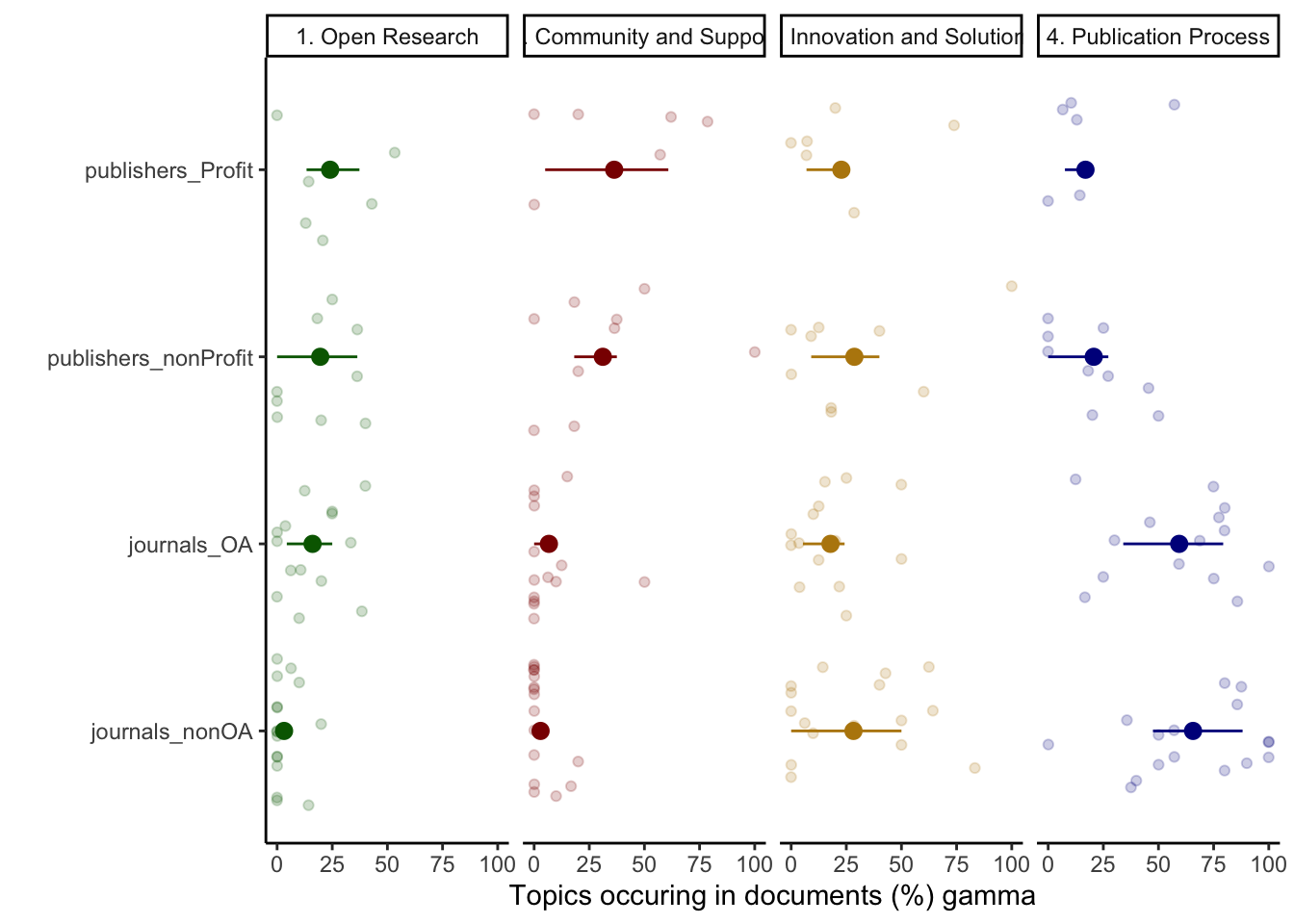

Past versions of unnamed-chunk-5-1.png

Version	Author	Date
c494066	zuzannazagrodzka	2023-12-02
8a4c1d4	zuzannazagrodzka	2023-11-10

# # UNCOMMENT TO SAVE FIGURES

figure_name <- paste0("./output/Figure_3A/Figure_3A.png")
png(file=figure_name,
  width= 3000, height= 2000, res=400)
  figure_topics
  dev.off()

quartz_off_screen 
                2 

Figure 3B

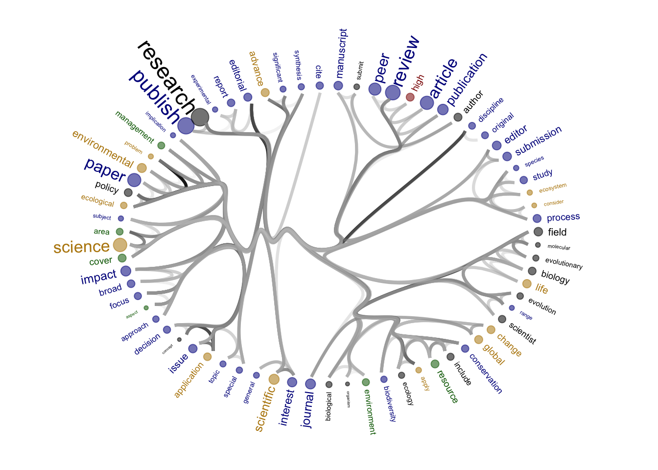
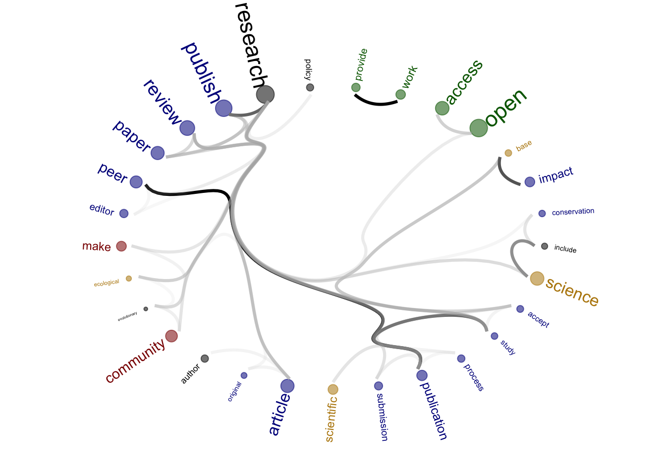
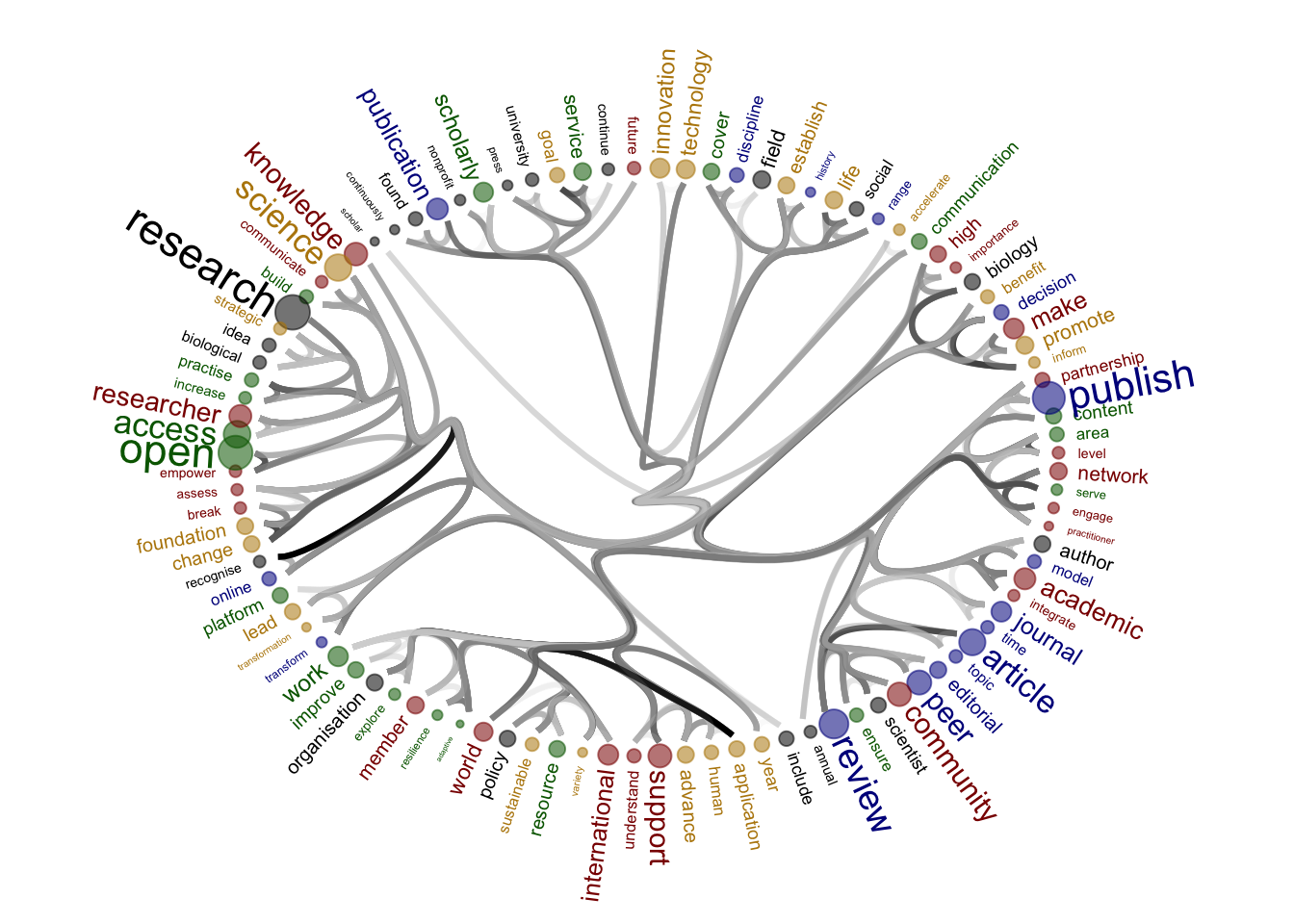
The figures will be reproduced but for subgroups: journals nonOa and OA, publishers for- and not-for-profit.

Source of the functions: https://www.markhw.com/blog/word-similarity-graphs We combined two methods - word similarity graphs and stm modelling) to be able visually explore topics and words’ connections in the aims and missions documents. We used the word similarity method (https://www.markhw.com/blog/word-similarity-graphs) to calculate similarities between words and later to be able to plot them with topic modeling score values (package stm)

The three primary steps are: 1. Calculating the similarities between words (Cosine matrix). 2. Formatting these similarity scores into a symmetric matrix, where the diagonal contains 0s and the off-diagonal cells are similarities between words.

3. Clustering nodes using a community detection algorithm (here: Walktrap algorithm) and plotting the data into circular hierarchical dendrograms for each of the stakeholder group separately (Figure 2B).

Libraries

Loading packages

# remotes::install_github('talgalili/dendextend')
library(dendextend)
library(igraph)
library(ggraph)
library(reshape2)
library(dplyr)
library(tidyverse)
library(tidytext)

Word similarity

Functions to create words similarities matrix.

• cosine_matrix
• Walktrap_topics

Source of the code: https://www.markhw.com/blog/word-similarity-graphs

# Cosine matrix
cosine_matrix <- function(tokenized_data, lower = 0, upper = 1, filt = 0) {
  
  if (!all(c("word", "id") %in% names(tokenized_data))) {
    stop("tokenized_data must contain variables named word and id")
  }
  
  if (lower < 0 | lower > 1 | upper < 0 | upper > 1 | filt < 0 | filt > 1) {
    stop("lower, upper, and filt must be 0 <= x <= 1")
  }
  docs <- length(unique(tokenized_data$id))
  
  out <- tokenized_data %>%
    count(id, word) %>%
    group_by(word) %>%
    mutate(n_docs = n()) %>%
    ungroup() %>%
    filter(n_docs <= (docs * upper) & n_docs > (docs * lower)) %>%
    select(-n_docs) %>%
    mutate(n = 1) %>%
    spread(word, n, fill = 0) %>%
    select(-id) %>%
    as.matrix() %>%
    lsa::cosine()
  
  filt <- quantile(out[lower.tri(out)], filt)
  out[out < filt] <- diag(out) <- 0
  out <- out[rowSums(out) != 0, colSums(out) != 0]
  
  return(out)
}


# Walktrap_topics

walktrap_topics <- function(g, ...) {
  wt <- igraph::cluster_walktrap(g, ...)
  
  membership <- igraph::cluster_walktrap(g, ...) %>% 
      igraph::membership() %>% 
      as.matrix() %>% 
      as.data.frame() %>% 
      rownames_to_column("word") %>% 
      arrange(V1) %>% 
      rename(group = V1)
  
  dendrogram <- stats::as.dendrogram(wt)
  
  return(list(membership = membership, dendrogram = dendrogram))
}

Data

# Importing data (created in `2_topic_modeling`)
# topics_df <- read.csv("./output/created_datasets/dataset_words_stm_5topics.csv")

# Importing dataset that we originally created and used in our analysis
topics_df <- read_feather(file = "./data/original_dataset_reproducibility_check/original_dataset_words_stm_5topics.arrow")

Creating a variable with the subgroups information

head(df_subgroups, 5)

# A tibble: 5 × 2
  name                             org_subgroups
  <chr>                            <chr>        
1 Africa Open Science and Hardware advocates    
2 Amelica                          advocates    
3 Bioline International            advocates    
4 Center for Open Science          advocates    
5 coalitionS                       advocates    

df_subgroups <- df_subgroups %>% 
  select("org_subgroups","name") %>% 
  distinct(.keep_all= FALSE)

# Keeping only subgroups I am interested in
topics_df <- topics_df %>% 
  filter(org_subgroups %in% c("publishers_nonProfit", "publishers_Profit", "journals_nonOA", "journals_OA"))

head(topics_df, 3)

# A tibble: 3 × 28
  txt        filename name  doc_type stakeholder sentence_doc orig_word word_mix
  <chr>      <chr>    <chr> <chr>    <chr>       <chr>        <chr>     <chr>   
1 "   Since… America… Amer… Aims     journals    American Na… inception incepti…
2 "   Since… America… Amer… Aims     journals    American Na… maintain… maintain
3 "   Since… America… Amer… Aims     journals    American Na… position  position
# ℹ 20 more variables: word <chr>, org_subgroups <chr>, mean_beta_t1 <dbl>,
#   mean_beta_t2 <dbl>, mean_beta_t3 <dbl>, mean_beta_t4 <dbl>,
#   mean_beta_t5 <dbl>, mean_score_t1 <dbl>, mean_score_t2 <dbl>,
#   mean_score_t3 <dbl>, mean_score_t4 <dbl>, mean_score_t5 <dbl>,
#   sum_beta_t1 <dbl>, sum_beta_t2 <dbl>, sum_beta_t3 <dbl>, sum_beta_t4 <dbl>,
#   sum_beta_t5 <dbl>, topic <int>, highest_mean_score <dbl>,
#   highest_mean_beta <dbl>

dim(topics_df)

[1] 6659   28

Running above functions for each substakeholder

stake_names <- unique(topics_df$org_subgroups)
count <- 1
figure_list <- vector()

for (stake in stake_names) {
  n <- count # number of the subsubgroups in the list
  stakeholder_name <- stake_names[n] # substakeholder's name
  
  # selecting data with the right name of the substakeholder
  dat <- topics_df %>%
  select(org_subgroups, sentence_doc, word) %>%
  rename(id = sentence_doc) %>% 
  filter(org_subgroups %in% stakeholder_name) %>% 
  select(-org_subgroups)
  ##################### 
  
  # Calculating similarity matrix
  cos_mat <- cosine_matrix(dat, lower = 0.050, upper = 1, filt = 0.9)
  
  # Getting words used in the network
  word_list_net <- rownames(cos_mat)
  grep("workflow", word_list_net)

  print(dim(cos_mat))
  
  # Creating a graph
  g <- graph_from_adjacency_matrix(cos_mat, mode = "undirected", weighted = TRUE)
  topics = walktrap_topics(g)
  print(stakeholder_name)
  plot(topics$dendrogram)

  subtrees <- partition_leaves(topics$dendrogram)
  leaves <- subtrees[[1]]  


  pathRoutes <- function(leaf) {
    which(sapply(subtrees, function(x) leaf %in% x))
  }

  paths <- lapply(leaves, pathRoutes)

  edges = NULL
  for(a in 1:length(paths)){
    # print(a)
    for(b in c(1:(length(paths[[a]])-1))){
     if(b == (length(paths[[a]])-1)){
        tmp_df = data.frame(
         from = paths[[a]][b],
         to = leaves[a]
       )
     } else {
        tmp_df = data.frame(
          from = paths[[a]][b],
          to = paths[[a]][b+1]
       )
     }
     edges = rbind(edges, tmp_df)
   }
  }


  connect = melt(cos_mat) # library reshape required
  colnames(connect) = c("from", "to", "value")
  connect = subset(connect, value != 0)

  # create a vertices data.frame. One line per object of our hierarchy
  vertices  <-  data.frame(
    name = unique(c(as.character(edges$from), as.character(edges$to))) 
  ) 
  # Let's add a column with the group of each name. It will be useful later to color points
  vertices$group  <-  edges$from[ match( vertices$name, edges$to ) ]


  #Let's add information concerning the label we are going to add: angle, horizontal adjustement and potential flip
  #calculate the ANGLE of the labels
  #vertices$id <- NA
  #myleaves <- which(is.na( match(vertices$name, edges$from) ))
  #nleaves <- length(myleaves)
  #vertices$id[ myleaves ] <- seq(1:nleaves)
  #vertices$angle <- 90 - 360 * vertices$id / nleaves

  # calculate the alignment of labels: right or left
  # If I am on the left part of the plot, my labels have currently an angle < -90
  #vertices$hjust <- ifelse( vertices$angle < -90, 1, 0)

  # flip angle BY to make them readable
  #vertices$angle <- ifelse(vertices$angle < -90, vertices$angle+180, vertices$angle)
  
  # replacing "group" value with the topic numer from the STM
  
  # Colour words by topic modelling topics (STM)
  # I have to change the group numbers in topics

  
  stm_top <- topics_df %>%
    select(org_subgroups, word, topic = topic) %>% 
    filter(org_subgroups %in% stakeholder_name) %>%
    select(-org_subgroups)
  

  stm_top$topic <- as.factor(stm_top$topic)
  stm_top <- unique(stm_top)


  # Removing group column and creating a new one based on the stm info
  vertices <- vertices

  vertices <- vertices %>% 
    left_join(stm_top, by = c("name" = "word")) %>% 
    select(-group) %>% 
    rename(group = topic)

  # Adding a beta value so I can use it in the graph
  stm_beta <- topics_df %>% 
    select(org_subgroups, word, beta = highest_mean_beta) %>% 
    filter(org_subgroups %in% stakeholder_name) %>%
    select(-org_subgroups)
  
  
  stm_beta <- unique(stm_beta)
  dim(stm_beta)

  vertices <- vertices %>% 
   left_join(stm_beta, by = c("name" = "word")) 


  vertices$beta_size = vertices$beta
  
  ##############################################################

  # Create a graph object
  mygraph <- igraph::graph_from_data_frame(edges, vertices=vertices)

  # The connection object must refer to the ids of the leaves:
  from  <-  match( connect$from, vertices$name)
  to  <-  match( connect$to, vertices$name)

  # Basic usual argument
  tmp_plt = ggraph(mygraph, layout = 'dendrogram', circular = T) + 
    geom_node_point(aes(filter = leaf, x = x*1.05, y=y*1.05, alpha=0.2), size =0, colour = "white") +
    #colour=group, size=value
          scale_colour_manual(values= c("dark green", "dark red", "darkgoldenrod", "dark blue", "black"), na.value = "black") +   
    geom_conn_bundle(data = get_con(from = from, to = to, col = connect$value), tension = 0.9, aes(colour = col, alpha = col+0.5), width = 1.1) +
    scale_edge_color_continuous(low="white", high="black") +
    # geom_node_text(aes(x = x*1.1, y=y*1.1, filter = leaf, label=name, angle = angle, hjust=hjust), size=5, alpha=1) +
    geom_node_text(aes(x = x*1.1, y=y*1.1, filter = leaf, label=name, colour = group, angle = 0, hjust = 0.5, size = beta_size),  alpha=1) +
    
     theme_void() +
    theme(
      legend.position="none",
      plot.margin=unit(c(0,0,0,0),"cm"),
    ) +
    expand_limits(x = c(-1.5, 1.5), y = c(-1.5, 1.5)) 

  g <- ggplot_build(tmp_plt)
  tmp_dat = g[[3]]$data
  tmp_dat$position = NA
  tmp_dat_a = subset(tmp_dat, x >= 0)
  tmp_dat_a = tmp_dat_a[order(-tmp_dat_a$y),]
  tmp_dat_a = subset(tmp_dat_a, !is.na(beta))
  tmp_dat_a$order = 1:nrow(tmp_dat_a)
  
  tmp_dat_b = subset(tmp_dat, x < 0)
  tmp_dat_b = tmp_dat_b[order(-tmp_dat_b$y),]
  tmp_dat_b = subset(tmp_dat_b, !is.na(beta))
  tmp_dat_b$order = (nrow(tmp_dat_a) +nrow(tmp_dat_b)) : (nrow(tmp_dat_a) +1)
  
  tmp_dat = rbind(tmp_dat_a, tmp_dat_b)
  
  vertices = left_join(vertices, tmp_dat[,c("name", "order")], by = c("name"))
  vert_save = vertices
  vertices = vert_save
  
  vertices$id <- NA
  vertices = vertices[order(vertices$order),]
  myleaves <- which(is.na( match(vertices$name, edges$from) ))
  nleaves <- length(myleaves)
  vertices$id[ myleaves ] <- seq(1:nleaves)
  vertices$angle <- 90 - 360 * vertices$id / nleaves
  
  # calculate the alignment of labels: right or left
  # If I am on the left part of the plot, my labels have currently an angle < -90
  vertices$hjust <- ifelse( vertices$angle < -90, 1, 0)
  
  # flip angle BY to make them readable
  vertices$angle <- ifelse(vertices$angle < -90, vertices$angle+180, vertices$angle)
  vertices = vertices[order(as.numeric(rownames(vertices))),]
  
  mygraph <- igraph::graph_from_data_frame(edges, vertices=vertices)
  
  figure_to_save <- ggraph(mygraph, layout = 'dendrogram', circular = T) + 
    geom_node_point(aes(filter = leaf, x = x*1.05, y=y*1.05, alpha=0.2, colour = group, size = beta_size)) +
    #colour=group, size=value
          scale_colour_manual(values= c("dark green", "dark red", "darkgoldenrod", "dark blue", "black"), na.value = "black") +   
    geom_conn_bundle(data = get_con(from = from, to = to, col = connect$value), tension = 0.99, aes(colour = col, alpha = col+0.5), width = 1.1) +
    scale_edge_color_continuous(low="grey90", high="black") +
    geom_node_text(aes(x = x*1.1, y=y*1.1, filter = leaf, label=name, colour = group, angle = angle, hjust = hjust, size = beta_size)) +
    
    theme_void() +
    theme(
      legend.position="none",
      plot.margin=unit(c(0,0,0,0),"cm"),
    ) +
    expand_limits(x = c(-1.5, 1.5), y = c(-1.5, 1.5))

  assign(paste0(stake_names[n], "_figure3B"), figure_to_save)
  # name_temp <- assign(paste0(stake_names[n], "_figure2b"), figure_to_save)
  figure_list <- append(figure_list, paste0(stake_names[n], "_figure3B"))
  
  print(figure_to_save)

  #####################
  count <-  count + 1 

}

[1] 71 71
[1] "journals_nonOA"

Warning: Using the `size` aesthetic in this geom was deprecated in ggplot2 3.4.0.
ℹ Please use `linewidth` in the `default_aes` field and elsewhere instead.
This warning is displayed once every 8 hours.
Call `lifecycle::last_lifecycle_warnings()` to see where this warning was
generated.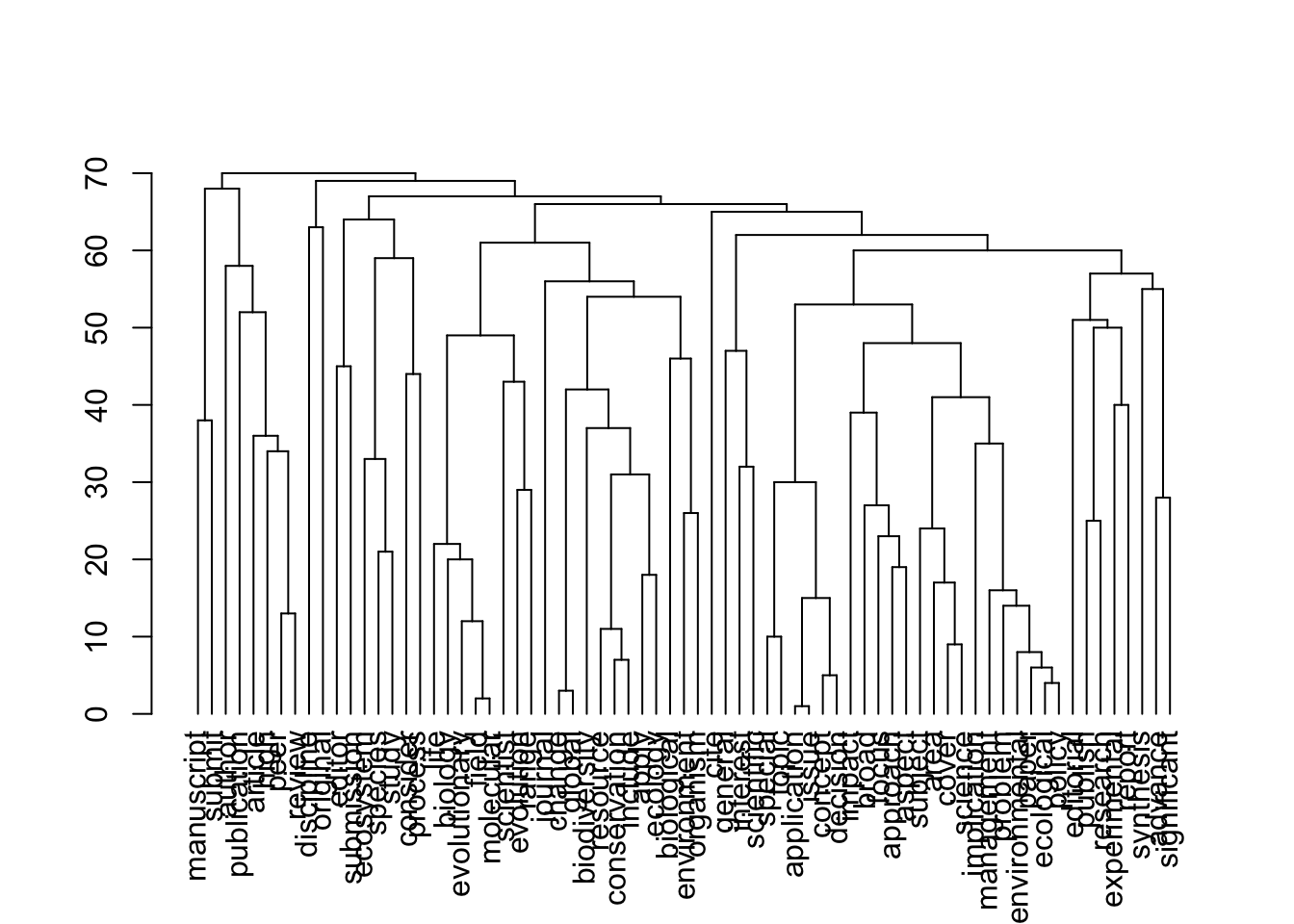

Past versions of unnamed-chunk-11-1.png

Version	Author	Date
8a4c1d4	zuzannazagrodzka	2023-11-10

Past versions of unnamed-chunk-11-2.png

Version	Author	Date
8a4c1d4	zuzannazagrodzka	2023-11-10

[1] 29 29
[1] "journals_OA"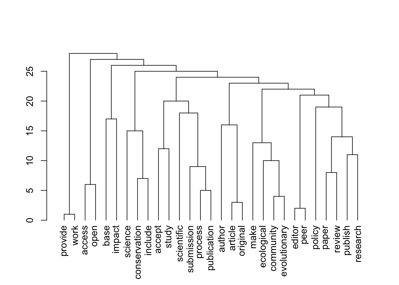

Past versions of unnamed-chunk-11-3.png

Version	Author	Date
8a4c1d4	zuzannazagrodzka	2023-11-10

Past versions of unnamed-chunk-11-4.png

Version	Author	Date
8a4c1d4	zuzannazagrodzka	2023-11-10

[1] 100 100
[1] "publishers_nonProfit"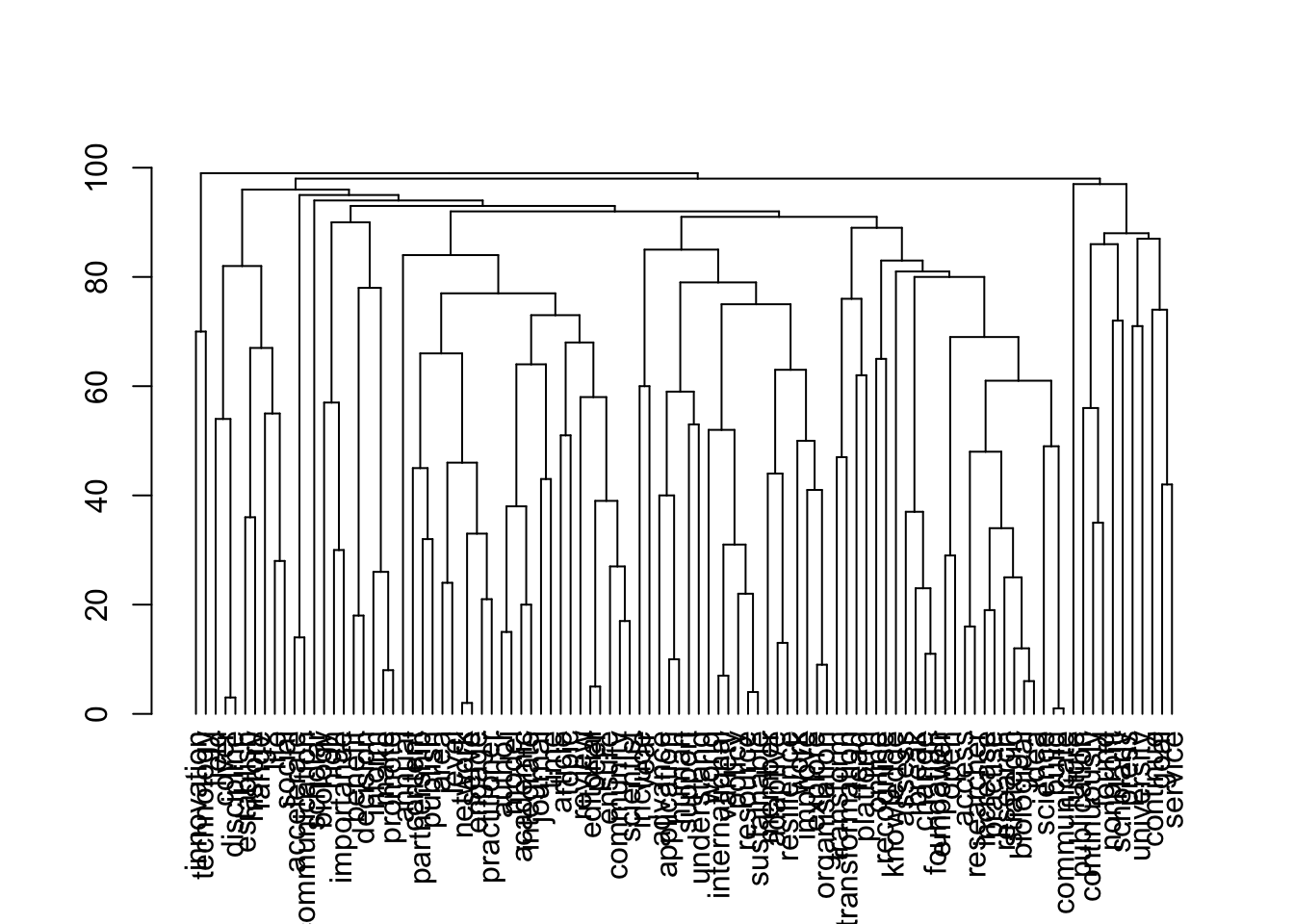

Past versions of unnamed-chunk-11-5.png

Version	Author	Date
c494066	zuzannazagrodzka	2023-12-02
8a4c1d4	zuzannazagrodzka	2023-11-10

Past versions of unnamed-chunk-11-6.png

Version	Author	Date
c494066	zuzannazagrodzka	2023-12-02
8a4c1d4	zuzannazagrodzka	2023-11-10

[1] 55 55
[1] "publishers_Profit"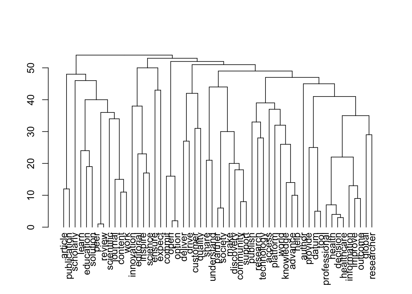

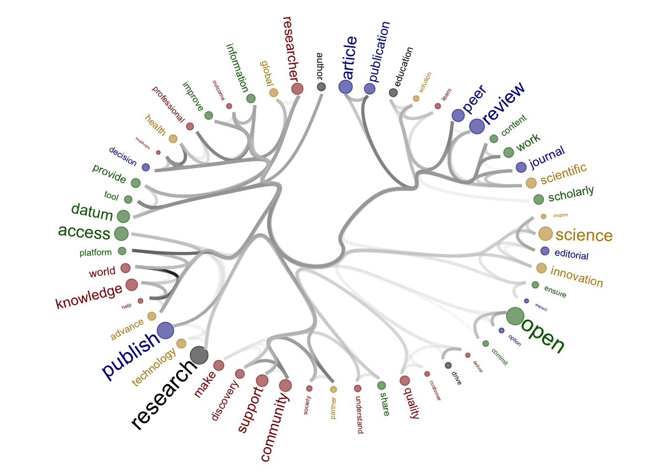
Past versions of unnamed-chunk-11-7.png

Version	Author	Date
c494066	zuzannazagrodzka	2023-12-02
8a4c1d4	zuzannazagrodzka	2023-11-10

Past versions of unnamed-chunk-11-8.png

Version	Author	Date
c494066	zuzannazagrodzka	2023-12-02
8a4c1d4	zuzannazagrodzka	2023-11-10

Figure production

# Saving figures individually 

figure_list

figure_name <- paste0("./output/Figure_3B/journals_nonOA_figure3B.png")
png(file=figure_name,
  width= 3000, height= 3000, res=400)
  journals_nonOA_figure3B
  dev.off()


figure_name <- paste0("./output/Figure_3B/journals_OA_figure3B.png")
png(file=figure_name,
  width= 3000, height= 3000, res=400)
  journals_OA_figure3B
  dev.off()
  
figure_name <- paste0("./output/Figure_3B/publishers_nonProfit_figure3B.png")
png(file=figure_name,
  width= 3000, height= 3000, res=400)
  publishers_nonProfit_figure3B
  dev.off()
  
  
figure_name <- paste0("./output/Figure_3B/publishers_Profit_figure3B.png")
png(file=figure_name,
  width= 3000, height= 3000, res=400)
  publishers_Profit_figure3B
  dev.off()

Session information

sessionInfo()

R version 4.3.1 (2023-06-16)
Platform: x86_64-apple-darwin20 (64-bit)
Running under: macOS Monterey 12.6

Matrix products: default
BLAS:   /Library/Frameworks/R.framework/Versions/4.3-x86_64/Resources/lib/libRblas.0.dylib 
LAPACK: /Library/Frameworks/R.framework/Versions/4.3-x86_64/Resources/lib/libRlapack.dylib;  LAPACK version 3.11.0

locale:
[1] en_US.UTF-8/en_US.UTF-8/en_US.UTF-8/C/en_US.UTF-8/en_US.UTF-8

time zone: Europe/London
tzcode source: internal

attached base packages:
[1] stats     graphics  grDevices utils     datasets  methods   base     

other attached packages:
 [1] tidytext_0.4.1    reshape2_1.4.4    ggraph_2.1.0      igraph_1.5.1     
 [5] dendextend_1.17.1 arrow_13.0.0.1    lubridate_1.9.3   forcats_1.0.0    
 [9] stringr_1.5.0     dplyr_1.1.3       purrr_1.0.2       readr_2.1.4      
[13] tidyr_1.3.0       tibble_3.2.1      ggplot2_3.4.3     tidyverse_2.0.0  
[17] workflowr_1.7.1  

loaded via a namespace (and not attached):
 [1] tidyselect_1.2.0   viridisLite_0.4.2  farver_2.1.1       viridis_0.6.4     
 [5] fastmap_1.1.1      tweenr_2.0.2       janeaustenr_1.0.0  promises_1.2.1    
 [9] digest_0.6.33      timechange_0.2.0   lifecycle_1.0.3    tokenizers_0.3.0  
[13] processx_3.8.2     magrittr_2.0.3     compiler_4.3.1     rlang_1.1.1       
[17] sass_0.4.7         tools_4.3.1        utf8_1.2.3         yaml_2.3.7        
[21] knitr_1.44         labeling_0.4.3     graphlayouts_1.0.2 bit_4.0.5         
[25] plyr_1.8.9         withr_2.5.1        grid_4.3.1         polyclip_1.10-6   
[29] fansi_1.0.4        git2r_0.32.0       colorspace_2.1-0   scales_1.2.1      
[33] MASS_7.3-60        cli_3.6.1          rmarkdown_2.25     crayon_1.5.2      
[37] generics_0.1.3     rstudioapi_0.15.0  httr_1.4.7         tzdb_0.4.0        
[41] cachem_1.0.8       ggforce_0.4.1      assertthat_0.2.1   vctrs_0.6.3       
[45] Matrix_1.5-4.1     jsonlite_1.8.7     lsa_0.73.3         callr_3.7.3       
[49] hms_1.1.3          bit64_4.0.5        ggrepel_0.9.4      jquerylib_0.1.4   
[53] glue_1.6.2         ps_1.7.5           stringi_1.7.12     gtable_0.3.4      
[57] later_1.3.1        munsell_0.5.0      pillar_1.9.0       htmltools_0.5.6   
[61] R6_2.5.1           tidygraph_1.2.3    rprojroot_2.0.3    evaluate_0.21     
[65] lattice_0.21-8     SnowballC_0.7.1    httpuv_1.6.11      bslib_0.5.1       
[69] Rcpp_1.0.11        gridExtra_2.3      whisker_0.4.1      xfun_0.40         
[73] fs_1.6.3           getPass_0.2-2      pkgconfig_2.0.3   

Session information

sessionInfo()

R version 4.3.1 (2023-06-16)
Platform: x86_64-apple-darwin20 (64-bit)
Running under: macOS Monterey 12.6

Matrix products: default
BLAS:   /Library/Frameworks/R.framework/Versions/4.3-x86_64/Resources/lib/libRblas.0.dylib 
LAPACK: /Library/Frameworks/R.framework/Versions/4.3-x86_64/Resources/lib/libRlapack.dylib;  LAPACK version 3.11.0

locale:
[1] en_US.UTF-8/en_US.UTF-8/en_US.UTF-8/C/en_US.UTF-8/en_US.UTF-8

time zone: Europe/London
tzcode source: internal

attached base packages:
[1] stats     graphics  grDevices utils     datasets  methods   base     

other attached packages:
 [1] tidytext_0.4.1    reshape2_1.4.4    ggraph_2.1.0      igraph_1.5.1     
 [5] dendextend_1.17.1 arrow_13.0.0.1    lubridate_1.9.3   forcats_1.0.0    
 [9] stringr_1.5.0     dplyr_1.1.3       purrr_1.0.2       readr_2.1.4      
[13] tidyr_1.3.0       tibble_3.2.1      ggplot2_3.4.3     tidyverse_2.0.0  
[17] workflowr_1.7.1  

loaded via a namespace (and not attached):
 [1] tidyselect_1.2.0   viridisLite_0.4.2  farver_2.1.1       viridis_0.6.4     
 [5] fastmap_1.1.1      tweenr_2.0.2       janeaustenr_1.0.0  promises_1.2.1    
 [9] digest_0.6.33      timechange_0.2.0   lifecycle_1.0.3    tokenizers_0.3.0  
[13] processx_3.8.2     magrittr_2.0.3     compiler_4.3.1     rlang_1.1.1       
[17] sass_0.4.7         tools_4.3.1        utf8_1.2.3         yaml_2.3.7        
[21] knitr_1.44         labeling_0.4.3     graphlayouts_1.0.2 bit_4.0.5         
[25] plyr_1.8.9         withr_2.5.1        grid_4.3.1         polyclip_1.10-6   
[29] fansi_1.0.4        git2r_0.32.0       colorspace_2.1-0   scales_1.2.1      
[33] MASS_7.3-60        cli_3.6.1          rmarkdown_2.25     crayon_1.5.2      
[37] generics_0.1.3     rstudioapi_0.15.0  httr_1.4.7         tzdb_0.4.0        
[41] cachem_1.0.8       ggforce_0.4.1      assertthat_0.2.1   vctrs_0.6.3       
[45] Matrix_1.5-4.1     jsonlite_1.8.7     lsa_0.73.3         callr_3.7.3       
[49] hms_1.1.3          bit64_4.0.5        ggrepel_0.9.4      jquerylib_0.1.4   
[53] glue_1.6.2         ps_1.7.5           stringi_1.7.12     gtable_0.3.4      
[57] later_1.3.1        munsell_0.5.0      pillar_1.9.0       htmltools_0.5.6   
[61] R6_2.5.1           tidygraph_1.2.3    rprojroot_2.0.3    evaluate_0.21     
[65] lattice_0.21-8     SnowballC_0.7.1    httpuv_1.6.11      bslib_0.5.1       
[69] Rcpp_1.0.11        gridExtra_2.3      whisker_0.4.1      xfun_0.40         
[73] fs_1.6.3           getPass_0.2-2      pkgconfig_2.0.3