7_For_and_not_for_profit_comparison_part_2
ZZ, APB, TFJ
2023-12-20
Last updated: 2023-12-20
Checks: 7 0
Knit directory:
workflowr-policy-landscape/
This reproducible R Markdown analysis was created with workflowr (version 1.7.1). The Checks tab describes the reproducibility checks that were applied when the results were created. The Past versions tab lists the development history.
Great! Since the R Markdown file has been committed to the Git repository, you know the exact version of the code that produced these results.
Great job! The global environment was empty. Objects defined in the global environment can affect the analysis in your R Markdown file in unknown ways. For reproduciblity it’s best to always run the code in an empty environment.
The command set.seed(20220505) was run prior to running
the code in the R Markdown file. Setting a seed ensures that any results
that rely on randomness, e.g. subsampling or permutations, are
reproducible.
Great job! Recording the operating system, R version, and package versions is critical for reproducibility.
Nice! There were no cached chunks for this analysis, so you can be confident that you successfully produced the results during this run.
Great job! Using relative paths to the files within your workflowr project makes it easier to run your code on other machines.
Great! You are using Git for version control. Tracking code development and connecting the code version to the results is critical for reproducibility.
The results in this page were generated with repository version a30bb03. See the Past versions tab to see a history of the changes made to the R Markdown and HTML files.
Note that you need to be careful to ensure that all relevant files for
the analysis have been committed to Git prior to generating the results
(you can use wflow_publish or
wflow_git_commit). workflowr only checks the R Markdown
file, but you know if there are other scripts or data files that it
depends on. Below is the status of the Git repository when the results
were generated:
Ignored files:
    Ignored:    .DS_Store
    Ignored:    .RData
    Ignored:    .Rhistory
    Ignored:    .Rproj.user/
    Ignored:    data/.DS_Store
    Ignored:    data/original_dataset_reproducibility_check/.DS_Store
    Ignored:    output/.DS_Store
    Ignored:    output/Figure_3B/.DS_Store
    Ignored:    output/created_datasets/.DS_Store

Untracked files:
    Untracked:  gutenbergr_0.2.3.tar.gz

Unstaged changes:
    Modified:   Policy_landscape_workflowr.R
    Modified:   data/original_dataset_reproducibility_check/original_cleaned_data.csv
    Modified:   data/original_dataset_reproducibility_check/original_dataset_words_stm_5topics.csv
    Modified:   output/Figure_3A/Figure_3A.png
    Modified:   output/created_datasets/cleaned_data.csv
Note that any generated files, e.g. HTML, png, CSS, etc., are not included in this status report because it is ok for generated content to have uncommitted changes.
These are the previous versions of the repository in which changes were
made to the R Markdown
(analysis/7_For_and_not_for_profit_comparison_part_2.Rmd)
and HTML
(docs/7_For_and_not_for_profit_comparison_part_2.html)
files. If you’ve configured a remote Git repository (see
?wflow_git_remote), click on the hyperlinks in the table
below to view the files as they were in that past version.
| File | Version | Author | Date | Message |
|---|---|---|---|---|
| html | 5c836ab | zuzannazagrodzka | 2023-12-07 | Build site. |
| Rmd | 8a502c9 | zuzannazagrodzka | 2023-12-07 | editing text |
| html | 9fec406 | zuzannazagrodzka | 2023-12-04 | Build site. |
| html | c494066 | zuzannazagrodzka | 2023-12-02 | Build site. |
| Rmd | 0f40512 | zuzannazagrodzka | 2023-12-02 | Update the file paths for all analysis and figures |
| Rmd | 4735075 | zuzannazagrodzka | 2023-12-02 | A new script that compares journals (variables: profit and access). Dictionary analysis, figures created |
There are questions we additionally addressed in the manuscript (part 2)
- What language do for-profit OA, for-profit nonOA, not-for-profit nonOA and not-for-profit OA journals use in their mission statements and aims?
- What organisations use more common language to the UNESCO Recommendations in Open Science and which use business words?
We conducted the same language analysis that were conducted on the main stakeholders groups to compare for-profit OA, for-profit nonOA, not-for-profit nonOA and not-for-profit OA journals.
The lists of the journals belonging to four categories we identified:
for_profit_no_oa (N = 11): “BioSciences”, “Biological Conservation”, “Conservation Biology”, “Ecological Applications”,“Ecology Letters”, “Ecology”, “Frontiers in Ecology and the Environment”, “Global Change Biology”, “Journal of Applied Ecology”, “Nature Ecology and Evolution”, “Trends in Ecology & Evolution”
no_profit_no_oa (N = 5): “American Naturalist”, “Annual Review of Ecology Evolution and Systematics”, “Evolution”, “Philosophical Transactions of the Royal Society B”, “Proceedings of the Royal Society B Biological Sciences”
for_profit_oa (N = 8): “Arctic, Antarctic, and Alpine Research”, “Biogeosciences”, “Conservation Letters”, “Diversity and Distributions”, “Ecology and Evolution”, “Evolutionary Applications”, “Neobiota”, “PeerJJournal”
no_profit_oa (N = 6): “Ecology and Society”, “Evolution Letters”, “Frontiers in Ecology and Evolution”, “Plos Biology”, “Remote Sensing in Ecology and Conservation”, “eLifeJournal”
R Step and Packages
# Clearing R
rm(list=ls())

# Libraries used for text/data analysis
library(tidyverse)
library(dplyr)
library(tidytext)

# Libraries used to create plots
library(ggplot2)

# Library to create a table when converting to html
library("kableExtra")

# Library to read an arrow file
library(arrow)
Import data
add column based on the name of the journal if its OA run by for profit or not-for-profit:
for_profit_no_oa: “BioSciences”, “Biological Conservation”, “Conservation Biology”, “Ecological Applications”,“Ecology Letters”, “Ecology”, “Frontiers in Ecology and the Environment”, “Global Change Biology”, “Journal of Applied Ecology”, “Nature Ecology and Evolution”, “Trends in Ecology & Evolution”
no_profit_no_oa: “American Naturalist”, “Annual Review of Ecology Evolution and Systematics”, “Evolution”, “Philosophical Transactions of the Royal Society B”, “Proceedings of the Royal Society B Biological Sciences”
for_profit_oa: “Arctic, Antarctic, and Alpine Research”, “Biogeosciences”, “Conservation Letters”, “Diversity and Distributions”, “Ecology and Evolution”, “Evolutionary Applications”, “Neobiota”, “PeerJJournal”
no_profit_oa: “Ecology and Society”, “Evolution Letters”, “Frontiers in Ecology and Evolution”, “Plos Biology”, “Remote Sensing in Ecology and Conservation”, “eLifeJournal”
Importing data
# Importing dataset created in "1a_Data_preprocessing.Rmd"
# df_corpuses <- read.csv(file = "./output/created_datasets/cleaned_data.csv")

# Importing dataset that we originally created and used in our analysis
df_corpuses <- read_feather(file = "./data/original_dataset_reproducibility_check/original_cleaned_data.arrow")

data_words <- df_corpuses

# Dictionary data
# Importing dictionary data that we originally created and used in our analysis
all_dict <- read.csv(file = "./data/original_dataset_reproducibility_check/original_freq_dict_total_all.csv")
Data Prep and Cleaning
# Data preparation

# Changing name of the dictionary variable
new_dictionary <- all_dict

## Getting a data set with the words
data_words <- df_corpuses

dim(data_words)
[1] 22822 10colnames(data_words) [1] "txt" "filename" "name" "doc_type"
[5] "stakeholder" "sentence_doc" "orig_word" "word_mix"
[9] "word" "org_subgroups"unique(data_words$org_subgroups)[1] "advocates" "funders" "journals_nonOA"
[4] "journals_OA" "publishers_nonProfit" "publishers_Profit"
[7] "repositories" "societies" # Merging and removing duplicates
data_words <- data_words %>%
rename(document = name) %>%
select(document, org_subgroups, word) %>%
left_join(new_dictionary, by = c("word" = "word")) %>% # merging
filter(org_subgroups %in% c("journals_nonOA", "journals_OA"))
data <- data_words
# Adding a column with a new variable
data$profit_access <- data$document
data$profit_access[data$profit_access%in% c("BioSciences", "Biological Conservation", "Conservation Biology", "Ecological Applications","Ecology Letters", "Ecology", "Frontiers in Ecology and the Environment", "Global Change Biology", "Journal of Applied Ecology", "Nature Ecology and Evolution", "Trends in Ecology & Evolution")] <- "for_profit_no_oa"
data$profit_access[data$profit_access%in% c("American Naturalist", "Annual Review of Ecology Evolution and Systematics", "Evolution", "Philosophical Transactions of the Royal Society B", "Proceedings of the Royal Society B Biological Sciences")] <- "no_profit_no_oa"
data$profit_access[data$profit_access%in% c("Arctic, Antarctic, and Alpine Research", "Biogeosciences", "Conservation Letters", "Diversity and Distributions", "Ecology and Evolution", "Evolutionary Applications", "Neobiota", "PeerJJournal")] <- "for_profit_oa"
data$profit_access[data$profit_access%in% c("Ecology and Society", "Evolution Letters", "Frontiers in Ecology and Evolution", "Plos Biology", "Remote Sensing in Ecology and Conservation", "eLifeJournal")] <- "no_profit_oa"
# # Check that all rows were replaced
#
# check <- data
#
# check <- check %>%
# select(profit_access) %>%
# group_by_all() %>%
# summarise(COUNT = n())
# check
data_words <- data# Adding a column with the type of journal and word together to allow merging later
data_words$stake_word <- paste(data_words$profit_access, "_", data_words$word)
# Adding a column with a document name and word together to allow merging later
data_words$doc_word <- paste(data_words$document, "_", data_words$word)
# Adding a column that will be used later to calculate the total of unique words in the document (dictionaries without removed words)
data_words$doc_pres <- 1
# Adding two columns that will be used later to calculate the total of unique words in the document (new dictionaries with removed common words)
# Replace NAs with 0 in all absence/presence columns
data_words_ND <- data_words %>%
mutate_at(vars(present_BUS, present_UNESCO, present_book, sum), ~replace_na(., 0)) # replacing NAs
head(data_words_ND,3)# A tibble: 3 × 12
document org_subgroups word present_in_dict present_BUS present_UNESCO
<chr> <chr> <chr> <int> <int> <int>
1 American Natur… journals_non… ince… 1 0 0
2 American Natur… journals_non… main… NA 0 0
3 American Natur… journals_non… posi… NA 0 0
# ℹ 6 more variables: present_book <int>, sum <int>, profit_access <chr>,
# stake_word <chr>, doc_word <chr>, doc_pres <dbl>colnames(data_words_ND) [1] "document" "org_subgroups" "word" "present_in_dict"
[5] "present_BUS" "present_UNESCO" "present_book" "sum"
[9] "profit_access" "stake_word" "doc_word" "doc_pres" ## Preparing columns used to creating ternary plots
# Select columns of my interest (stakeholders) and aggregate
data_words_ND <- data_words_ND %>%
select(document, profit_access, word, present_BUS, present_UNESCO, present_book, doc_pres, sum) # selecting columns, sum - column with the information about in how many dictionaries a certain word occurs
df_sum_pres_ND <- aggregate(x = data_words_ND[,4:8], by = list(data_words_ND$document), FUN = sum, na.rm = TRUE)
# By doing aggregate I lost info about the org_subgroups the doc come from, I want to add it
df_doc_ord <- data_words_ND %>%
select(document, profit_access) %>%
distinct(document, .keep_all = TRUE)
df_sum_pres_ND <- df_sum_pres_ND %>%
left_join(df_doc_ord, by = c("Group.1" = "document")) %>%
rename(document = Group.1)
# Creating % columns in a new df_sum_proc_ND data frame
df_sum_proc_ND <- df_sum_pres_ND
# View(df_sum_proc_ND)
df_sum_proc_ND$proc_BUS <-df_sum_proc_ND$present_BUS/df_sum_proc_ND$doc_pres*100
df_sum_proc_ND$proc_UNESCO <- df_sum_proc_ND$present_UNESCO/df_sum_proc_ND$doc_pres*100
df_sum_proc_ND$proc_book <- df_sum_proc_ND$present_book/df_sum_proc_ND$doc_pres*100
# Additional information about the data
# Stakeholders (2 from each of the stakeholders) that shared the highest no of words with UNESCO recommendation
UNESCO_stak_top <- df_sum_proc_ND %>%
group_by(profit_access) %>%
arrange(desc(proc_UNESCO)) %>%
slice_head(n=2) %>%
select(profit_access, document, proc_UNESCO)
UNESCO_stak_top %>%
kbl(caption = "Stakeholders that shared the higest no of words with UNESCO recommendation:") %>%
kable_classic("hover", full_width = T)| profit_access | document | proc_UNESCO |
|---|---|---|
| for_profit_no_oa | Ecology Letters | 9.677419 |
| for_profit_no_oa | Frontiers in Ecology and the Environment | 8.411215 |
| for_profit_oa | Conservation Letters | 8.823529 |
| for_profit_oa | Diversity and Distributions | 7.009346 |
| no_profit_no_oa | Evolution | 3.030303 |
| no_profit_no_oa | Proceedings of the Royal Society B Biological Sciences | 2.678571 |
| no_profit_oa | Frontiers in Ecology and Evolution | 13.636364 |
| no_profit_oa | Remote Sensing in Ecology and Conservation | 6.796117 |
# Stakeholders (2 from each of the stakeholders) that shared the highest no of words with business dictionary

business_stak_top <- df_sum_proc_ND %>%
  group_by(profit_access) %>%
  arrange(desc(proc_BUS)) %>%
  slice_head(n=2) %>%
  select(profit_access, document, proc_BUS)

business_stak_top %>%
  kbl(caption = "Stakeholders that shared the higest no of words with business dictionary:") %>%
kable_classic("hover", full_width = T)| profit_access | document | proc_BUS |
|---|---|---|
| for_profit_no_oa | Ecology | 8.212560 |
| for_profit_no_oa | Global Change Biology | 7.142857 |
| for_profit_oa | Biogeosciences | 5.917160 |
| for_profit_oa | Evolutionary Applications | 5.421687 |
| no_profit_no_oa | Evolution | 21.212121 |
| no_profit_no_oa | Annual Review of Ecology Evolution and Systematics | 8.108108 |
| no_profit_oa | Evolution Letters | 6.349206 |
| no_profit_oa | Remote Sensing in Ecology and Conservation | 5.825243 |
# Stakeholders (2 from each of the stakeholders) that shared the highest no of words with book dictionary (control)

book_stak_top <-  df_sum_proc_ND %>%
  group_by(profit_access) %>%
  arrange(desc(proc_book)) %>%
  slice_head(n=2) %>%
  select(profit_access, document, proc_book)

book_stak_top %>%
  kbl(caption = "Stakeholders that shared the higest no of words with book dictionary (control):") %>%
kable_classic("hover", full_width = T)| profit_access | document | proc_book |
|---|---|---|
| for_profit_no_oa | Conservation Biology | 18.81188 |
| for_profit_no_oa | Trends in Ecology & Evolution | 18.07229 |
| for_profit_oa | Ecology and Evolution | 17.82407 |
| for_profit_oa | Arctic, Antarctic, and Alpine Research | 15.75092 |
| no_profit_no_oa | Annual Review of Ecology Evolution and Systematics | 16.21622 |
| no_profit_no_oa | Philosophical Transactions of the Royal Society B | 12.61261 |
| no_profit_oa | Evolution Letters | 22.22222 |
| no_profit_oa | Remote Sensing in Ecology and Conservation | 20.38835 |
Creating graphs
no <- nrow(df_sum_proc_ND)
no
[1] 30# Plotting them separately book
df_sum_proc_ND_book = data.frame(
document = rep(df_sum_proc_ND$document,1),
profit_access = rep(df_sum_proc_ND$profit_access,1),
type = c(rep("Book",no)),
perc = c(df_sum_proc_ND$proc_book),
perc2 = c(df_sum_proc_ND$proc_book))
sum_df_sum_proc_ND_book =
df_sum_proc_ND_book %>%
group_by(profit_access, type) %>%
# dplyr::summarise(perc = mean(perc), SD = sd(perc2))
dplyr::summarise(perc = median(perc), SD = sd(perc2))`summarise()` has grouped output by 'profit_access'. You can override using the
`.groups` argument.fig_book <- ggplot() +
geom_point(data = df_sum_proc_ND_book, aes(x = perc, y = profit_access), alpha = 0.1, position = position_jitter()) +
geom_pointrange(data = sum_df_sum_proc_ND_book, aes(x = perc, xmin = perc - SD, xmax = perc + SD, y = profit_access)) +
facet_grid(type~.) +
labs(x = "Document words occuring in dictionary (%)", y = "") +
scale_colour_discrete(guide = "none") +
theme_classic()
fig_book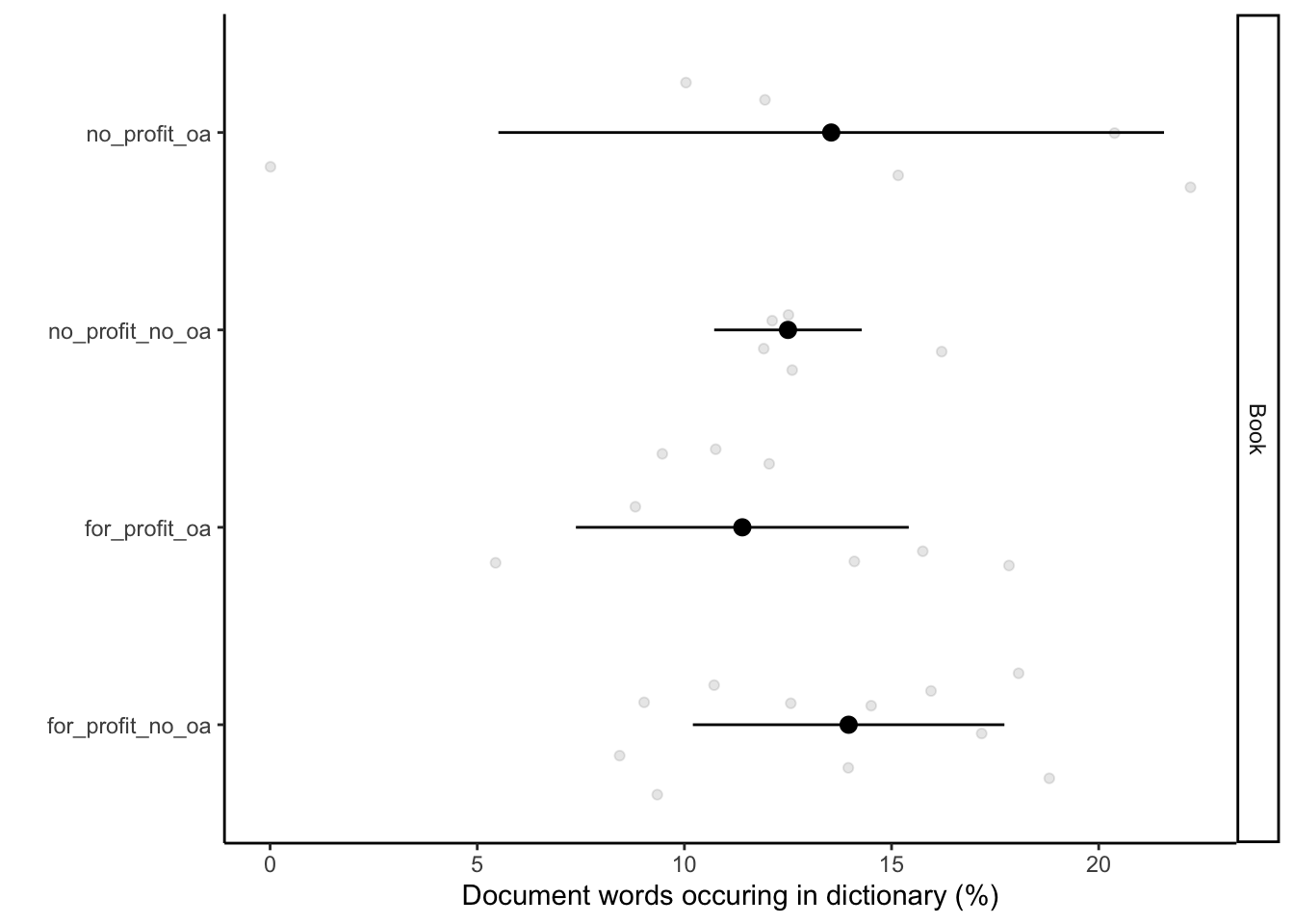
| Version | Author | Date |
|---|---|---|
| c494066 | zuzannazagrodzka | 2023-12-02 |
# Saving the figure
# UNCOMMENT TO SAVE THE FIGURE
figure_name <- paste0("./output/Figure_4C/Figure_4C_book.png")
ggsave(filename = figure_name, fig_book  + theme_bw(base_size = 5),
     width = 10, height = 5, dpi = 600, units = "in", device='png')


# Plotting them separately Business
df_sum_proc_ND_BUS = data.frame(
  document = rep(df_sum_proc_ND$document,1),
  profit_access = rep(df_sum_proc_ND$profit_access,1),
  type = c(rep("Business",no)),
  perc = c(df_sum_proc_ND$proc_BUS),
  perc2 = c(df_sum_proc_ND$proc_BUS))

sum_df_sum_proc_ND_BUS =
  df_sum_proc_ND_BUS %>%
  group_by(profit_access, type) %>%
  # dplyr::summarise(perc = mean(perc), SD = sd(perc2))
  dplyr::summarise(perc = median(perc), SD = sd(perc2))
`summarise()` has grouped output by 'profit_access'. You can override using the
`.groups` argument.fig_bus <- ggplot() +
geom_point(data = df_sum_proc_ND_BUS, aes(x = perc, y = profit_access), alpha = 0.1, position = position_jitter()) +
geom_pointrange(data = sum_df_sum_proc_ND_BUS, aes(x = perc, xmin = perc - SD, xmax = perc + SD, y = profit_access)) +
facet_grid(type~.) +
labs(x = "Document words occuring in dictionary (%)", y = "") +
scale_colour_discrete(guide = "none") +
theme_classic()
fig_bus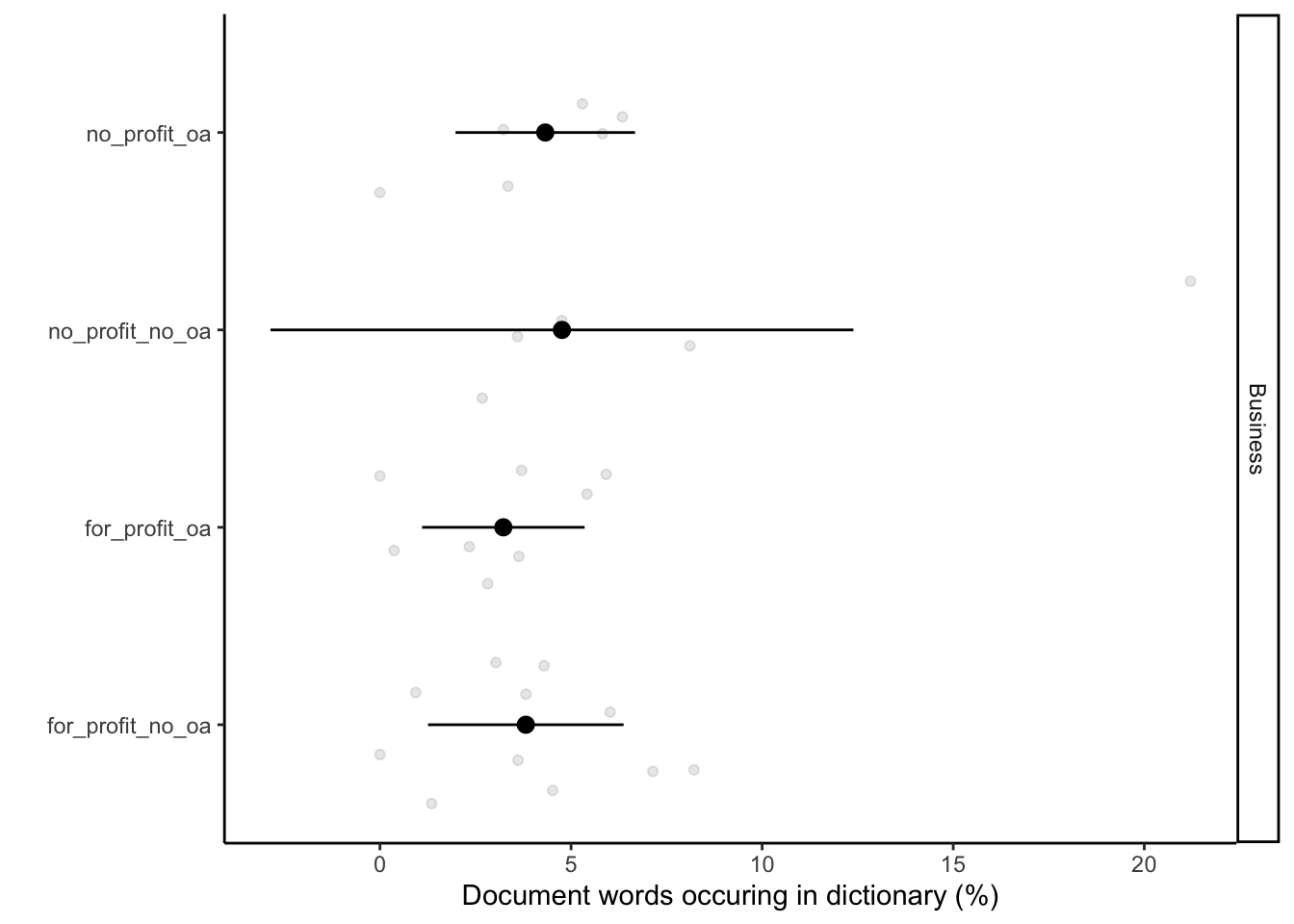
| Version | Author | Date |
|---|---|---|
| c494066 | zuzannazagrodzka | 2023-12-02 |
# Saving the figure
# UNCOMMENT TO SAVE THE FIGURE
figure_name <- paste0("./output/Figure_4C/Figure_4C_bus.png")
ggsave(filename = figure_name, fig_bus  + theme_bw(base_size = 5),
     width = 10, height = 5, dpi = 600, units = "in", device='png')


# Plotting them separately UNESCO
df_sum_proc_ND_UNESCO = data.frame(
  document = rep(df_sum_proc_ND$document,1),
  profit_access = rep(df_sum_proc_ND$profit_access,1),
  type = c(rep("UNESCO",no)),
  perc = c(df_sum_proc_ND$proc_UNESCO),
  perc2 = c(df_sum_proc_ND$proc_UNESCO))

sum_df_sum_proc_ND_UNESCO =
  df_sum_proc_ND_UNESCO %>%
  group_by(profit_access, type) %>%
  # dplyr::summarise(perc = mean(perc), SD = sd(perc2))
  dplyr::summarise(perc = median(perc), SD = sd(perc2))
`summarise()` has grouped output by 'profit_access'. You can override using the
`.groups` argument.fig_unesco <- ggplot() +
geom_point(data = df_sum_proc_ND_UNESCO, aes(x = perc, y = profit_access), alpha = 0.1, position = position_jitter()) +
geom_pointrange(data = sum_df_sum_proc_ND_UNESCO, aes(x = perc, xmin = perc - SD, xmax = perc + SD, y = profit_access)) +
facet_grid(type~.) +
labs(x = "Document words occuring in dictionary (%)", y = "") +
scale_colour_discrete(guide = "none") +
theme_classic()
fig_unesco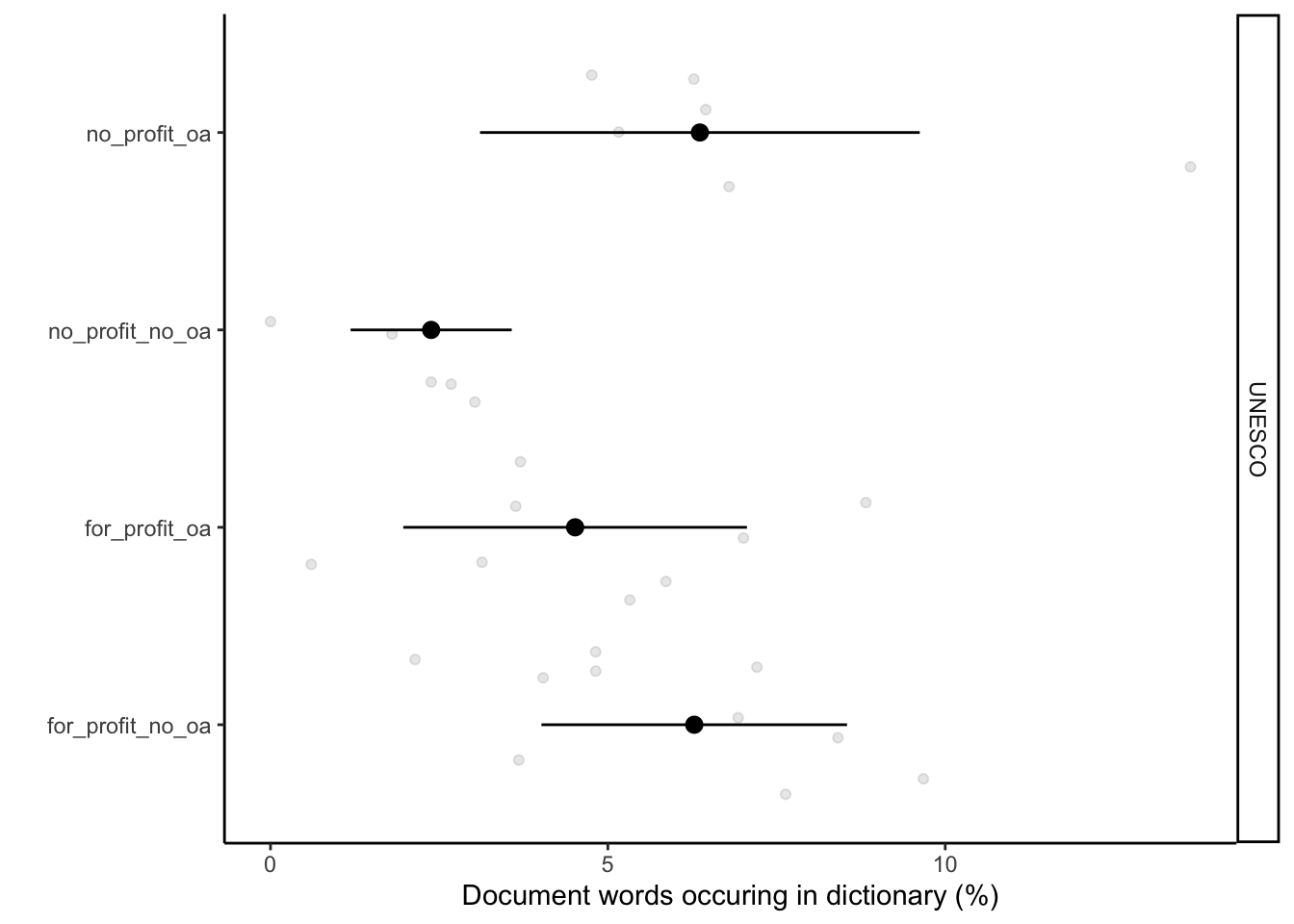
| Version | Author | Date |
|---|---|---|
| c494066 | zuzannazagrodzka | 2023-12-02 |
# Saving the figure
# UNCOMMENT TO SAVE THE FIGURE
figure_name <- paste0("./output/Figure_4C/Figure_4C_unesco.png")
ggsave(filename = figure_name, fig_unesco  + theme_bw(base_size = 5),
     width = 10, height = 5, dpi = 600, units = "in", device='png')
Session information
sessionInfo()R version 4.3.1 (2023-06-16)
Platform: x86_64-apple-darwin20 (64-bit)
Running under: macOS Monterey 12.6
Matrix products: default
BLAS: /Library/Frameworks/R.framework/Versions/4.3-x86_64/Resources/lib/libRblas.0.dylib
LAPACK: /Library/Frameworks/R.framework/Versions/4.3-x86_64/Resources/lib/libRlapack.dylib; LAPACK version 3.11.0
locale:
[1] en_US.UTF-8/en_US.UTF-8/en_US.UTF-8/C/en_US.UTF-8/en_US.UTF-8
time zone: Europe/London
tzcode source: internal
attached base packages:
[1] stats graphics grDevices utils datasets methods base
other attached packages:
[1] arrow_13.0.0.1 kableExtra_1.3.4 tidytext_0.4.1 lubridate_1.9.3
[5] forcats_1.0.0 stringr_1.5.0 dplyr_1.1.3 purrr_1.0.2
[9] readr_2.1.4 tidyr_1.3.0 tibble_3.2.1 ggplot2_3.4.3
[13] tidyverse_2.0.0 workflowr_1.7.1
loaded via a namespace (and not attached):
[1] gtable_0.3.4 xfun_0.40 bslib_0.5.1 processx_3.8.2
[5] lattice_0.21-8 callr_3.7.3 tzdb_0.4.0 vctrs_0.6.3
[9] tools_4.3.1 ps_1.7.5 generics_0.1.3 fansi_1.0.4
[13] highr_0.10 janeaustenr_1.0.0 pkgconfig_2.0.3 tokenizers_0.3.0
[17] Matrix_1.5-4.1 assertthat_0.2.1 webshot_0.5.5 lifecycle_1.0.3
[21] farver_2.1.1 compiler_4.3.1 git2r_0.32.0 textshaping_0.3.6
[25] munsell_0.5.0 getPass_0.2-2 httpuv_1.6.11 htmltools_0.5.6
[29] SnowballC_0.7.1 sass_0.4.7 yaml_2.3.7 later_1.3.1
[33] pillar_1.9.0 jquerylib_0.1.4 whisker_0.4.1 cachem_1.0.8
[37] tidyselect_1.2.0 rvest_1.0.3 digest_0.6.33 stringi_1.7.12
[41] labeling_0.4.3 rprojroot_2.0.3 fastmap_1.1.1 grid_4.3.1
[45] colorspace_2.1-0 cli_3.6.1 magrittr_2.0.3 utf8_1.2.3
[49] withr_2.5.1 scales_1.2.1 promises_1.2.1 bit64_4.0.5
[53] timechange_0.2.0 rmarkdown_2.25 httr_1.4.7 bit_4.0.5
[57] ragg_1.2.5 hms_1.1.3 evaluate_0.21 knitr_1.44
[61] viridisLite_0.4.2 rlang_1.1.1 Rcpp_1.0.11 glue_1.6.2
[65] xml2_1.3.5 svglite_2.1.2 rstudioapi_0.15.0 jsonlite_1.8.7
[69] R6_2.5.1 systemfonts_1.0.4 fs_1.6.3