6 Designs for testing for interactions: the two-way ANOVA and factorial designs.
6.1 Introducing Interactions
In the previous sections, and the 1-way ANOVA module in week 7, we have focused on a single explanatory variable. In week 7, it was the parasite factor. In the previous chapters focusing on yield, it was the herbicide treatment. In these cases, the question we are asking is about a single, main effect. However, there are many cases where we design experiments that might have two variables. For example, we may be interesting in the effect of parasite on growth but also whether this effect varies by the amount of food available. Or we might be interested in the yeild of a crop as a function of the herbicide, but also of soil water content. Or we might be interested in the rate of cell division as a function of a growth hormon, but also of whether this varies by the presence of a calcium blocker. In all of these cases we are asking a question about whether the effect of one treatment varies by the level of another. Thus, our question here is about an interaction.
Before jumping into an example, let’s introduce a simple statement that forms the core of both asking and interpreting interactions.
If there is an interaction between two explanatory variables, X and Z, on our response variable Y, then:
The effect of X on Y varies by Z. OR The effect of X on Y depends on Z.
This use of varies by OR depends on defines context dependency and that’s what defines interactions.
6.1.1 An Example with CO2 and UV-B solar radiation impact on plant growth in the artic.
Context: an arctic tundra study Increasing ultraviolet-B (+UV-B) radiation from ozone depletion (the arctic ozone hole) Increasing atmospheric CO2 (+CO2) from anthropogenic emissions For plants: UV-B potentially harmful, +CO2 potentially beneficial Therefore +CO2 could alleviate UV-B damage impacts.
Hypothesis
The effect of UV-B radiation on growth will depend on levels of CO2
Predictions:
+UV-B radiation will reduce the growth of arctic plants +CO2 will increase the growth of arctic plants +UV-B radiation impacts will be less under +CO2
What is unique about this context, hypothesis, and predictions?
It’s the presentation of CO2 and UVB in the same statement and the use of words like “the effect of X will alleviate the impacts of Y” and words like “the effects of X will be less under Y”. These words and phrases reflect the context dependency of the effects of treatment levels.
Thus, to restate what we introduced above…. when we talk about interactions, we can rely on a very simple vocabulary that is independent of the actual treatment levels: we can always describe an interaction like this:
The effect of X on Y depends on Z.
or
The effect of X on Y varies by Z.
In this ‘rubric’, Y is the response variable, and X and Z are explanatory, independent variables. So, in our example above,
the effect of CO2 on plant biomass yield depends on UV-B radiation levels.
OR
the effect of CO2 on plant biomass yield varies with UV-B radiation levels.
This simple phrasing describes any interaction.
6.1.1.1 Numerical example for emphasis
Let’s imagine the following situation. The folowing three numbers are what we call Main Effects:
Control = 20g Yield UV-B = 10g Yield C02 = 29g Yield
These numbers allow us to calculate the Additive Effect, where the effect of both CO2 and UV-B is simply estimated by adding the two independent effects together:
ADDITIVE RESULT: C02 + UV-B = 39g Yield
However, this additive outcome may not be what happens. Imagine if there were Synergy - the effects are more than the sum of the independent effects - or Antagonism - the effects are less than expected because one offsets the other.
SYNERGISTIC RESULT: C02 + UV-B = 60g Yield ANTAGONISTIC RESULT: C02 + UV-B = 19g Yield
6.1.1.2 The Factorial Design: Why Study Interactions?
The UV-B and C02 experiment could be thought of as two experiments – a Control vs UV-B and a Control vs C02 experiment. If we combine these we get a Factorial Experiment where we can actually estimate whether there is an interaction, and whether it is synergy or antagonism. In the factorial design for this example, there are four treatment levels and all combinations of all treatments.
- Control
- UV-B
- C02
- UV-B + C02
Some of you may be thinking that we could simply treat each of these treatment levels indepdently, as unique treatments levels - e.g. the one-way ANOVA. But we don’t. We design and analyse the data we collect in a two-way analysis - a factorial design. Two-way ANOVA is the design
Factorial treatments have two main advantages over the 1-way approach.
When factors DO interact – so the effect of C02 depends on UV-B – then we can estimate the interaction - the dependency. One-way designs cannot do this, and can lead to serious misunderstandings (because we are assuming that the effect of one thing DOES NOT depend on the other).
Furthermore, when factors DON’T interact, factorial designs are more precise (smaller error variance) at estimating the main (non-interacting effects) than one-way designs experiments.
Hence ALWAYS use factorial designs when your experimental design contains the interaction (when you are asking the question that includes the word(s) depends or varies by!
6.2 A Factorial Design and the Two-Way ANOVA
The following dataset plantYield_factorial contains two observation columns - yield_ind are data where there is NO INTERACTION. yield_int are data where there are an interaction. We will use both of these to showcase how to work the 2-way ANOVA and the analysis of a factorial design.
We note that these data have replication and randomisation. There are four replicate plants/plots allocated randomly to each of the four treatment combinations.
Here is the evidence of the factorial design
xtabs(~UVB+CO2, data = plantYield_factorial)## CO2
## UVB Con CO2+
## Con 4 4
## UVB+ 4 46.2.1 Plot the factorial design!
Here we combine some dplyr magic (calculating means in each group - NOTE that there are two grouping variables!), some ggplot magic (adding the lines connecting the means on top of the raw data) and the beauty of patchwork, the package for plot layouts.
Our goal here is to plot the data that does not have the interaction next to a plot of the data that does have the interaction.
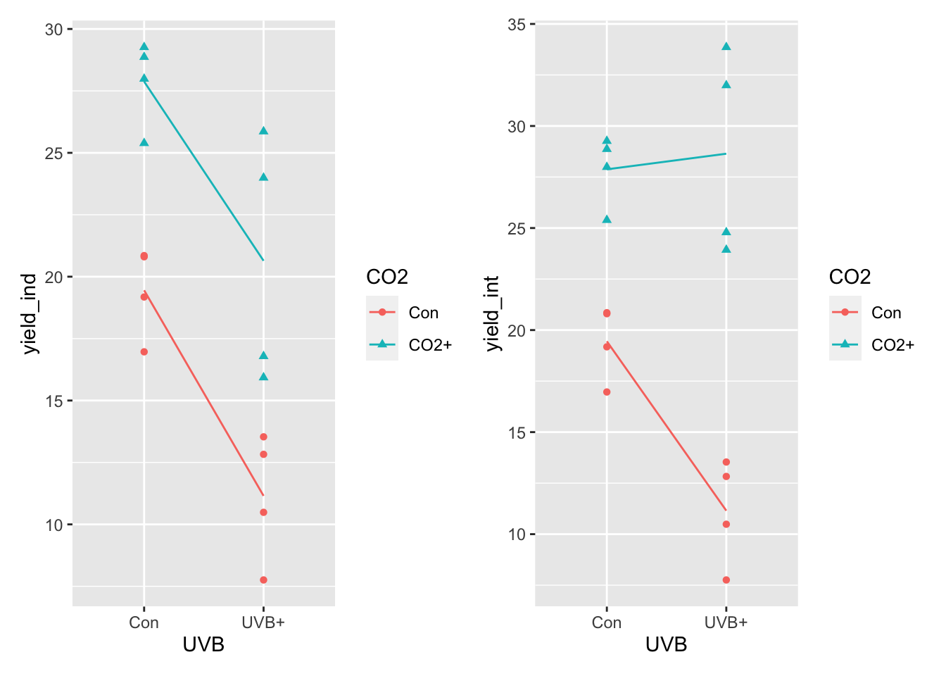
Given what you’ve read above, you should be able to fill in these blanks:
What you see above on the left, is a pattern that suggest that the effect of ______ on ________ does not vary by ________.
In contrast, on the right the pattern suggests that the effect of ______ on ________ ________ by ________:
6.2.2 How to analyse and interpret the factorial design
As with the plotting, we now analyse each data set.
We also make a mistake of analysing the data that has an interaction with a model that does not specify this interaction.
We are thus making three models. A model of the no interaction data without specifying and interaction, a model of the interaction data without specifying and interaction and a model of the interaction data with and interaction specified. This second model is incorrect, but fitting it helps illuminate why you should fit the interaction if your design contains the potential for an interaction (a factorial design).
An Important Note on what + and * mean in models. In the below model specification, you will see CO2 + UVB and CO2 * UVB. Using the vocabulary from above, CO2 + UVB is specifying independent additive effects. In the ANOVA table produced by anova(), there will be three lines: one for CO2, one for UVB and one for residuals. In contrast, CO2 * UVB produces four lines of output in the ANOVA table. We say that CO2 * UVB expands to include the main, independent effects of CO2 and UVB, but also the interaction between them. So CO2 * UVB == CO2 + UVB + CO2:UVB where the last term is the interaction. Thus, there are four lines reported: one for CO2, one for UVB, one for the interaction and one for residuals.
# A Correct model with no interaction on data with no interaction
int_mod_1 <- lm(yield_ind ~ CO2 + UVB, data = plantYield_factorial)

# A Correct model with interaction where the should be an interaction
int_mod_2 <- lm(yield_int ~ CO2 * UVB, data = plantYield_factorial)

# THE WRONG MODEL: model without interaction, on data that should use the interaction
int_mod_3 <- lm(yield_int ~ CO2 + UVB, data = plantYield_factorial)

anova(int_mod_1) # Good model, no interaction in the data and none in the model
## Analysis of Variance Table
##
## Response: yield_ind
## Df Sum Sq Mean Sq F value Pr(>F)
## CO2 1 321.00 321.00 35.905 4.504e-05 ***
## UVB 1 241.27 241.27 26.987 0.0001726 ***
## Residuals 13 116.22 8.94
## ---
## Signif. codes: 0 '***' 0.001 '**' 0.01 '*' 0.05 '.' 0.1 ' ' 1
anova(int_mod_2) # Good model, interaction in the data and interaction in the model## Analysis of Variance Table
##
## Response: yield_int
## Df Sum Sq Mean Sq F value Pr(>F)
## CO2 1 671.67 671.67 70.0311 2.364e-06 ***
## UVB 1 56.75 56.75 5.9165 0.03159 *
## CO2:UVB 1 82.15 82.15 8.5654 0.01268 *
## Residuals 12 115.09 9.59
## ---
## Signif. codes: 0 '***' 0.001 '**' 0.01 '*' 0.05 '.' 0.1 ' ' 1
anova(int_mod_3) # Bad model, interaction in the data, but failure to specify in the model## Analysis of Variance Table
##
## Response: yield_int
## Df Sum Sq Mean Sq F value Pr(>F)
## CO2 1 671.67 671.67 44.269 1.58e-05 ***
## UVB 1 56.75 56.75 3.740 0.07519 .
## Residuals 13 197.24 15.17
## ---
## Signif. codes: 0 '***' 0.001 '**' 0.01 '*' 0.05 '.' 0.1 ' ' 1Let’s focus on model 2 and how we interpret this. The ANOVA table now has multiple rows. We saw this before with the block design. The important thing to note here is that the table is now read sequentially. We first note that CO2 explains \(671.67\) units of variation (Mean Sq) in plant Yield. Having captured this variation, we then note that UVB captures \(56.75\) additional units. Then, having capture the variation caused directly by CO2 and UVB, we now see that the interaction - asking whether the effect of CO2 varies by UVB - explains an additional \(82.15\) units. And… there are \(9.59\) units of unexplained variation.
Great. So, remember as well how we calculate the F-value. In the ANOVA (categorial variable) framework, the F-value is the ratio of variance explained by the factor relative to the residual variation. So that’s where the F values come from…. And recall that BIG F-values indicate that more variation is allocated to the treatment levels, versus what’s left over. The bigger the numerator value relative to the residual denominator, the more variation this term has explained.
In this experimental design, and any like it, one must remember that there is actually a single question, and it does not related to the independent main effects.It relates only to the interaction term: we designed this experiment to test the hypothesis that the effect of CO2 on yield varies by UVB. There is only a single choice of answer - yes or no. In this case (Model 2), having captured variation with each independent effect, there is still a large amount of variation captured by ‘allowing’ the effects of each to vary by the other. Under a null hypothesis that these two variables to not interact (do not depend on each other), getting a Mean square estimate of \(82.15\) relative to the residual of \(9.59\) is very unlikely. So we reject the null!
Spend some time investigating what has happened with model 2 and model 3 and recall that ONLY ONE OF THEM IS CORRECT, regardless of whether the data look like the left or right panel above. Note the differences in the outputs. Note what we infer if we model the interaction data incorrectly.
There is no free lunch.
You must understand your data and your question and you must fit the model that correctly matches your design! In this case, there really is only one model you should fit. It is model 2. EVEN if the data look like the left panel, with no interaction, this experiment was designed to test the hypothesis that the effect of CO2 varies by UVB. You can only accept or reject the null hypothesis of no interaction by fitting model 2. You can not guess the right model from the picture. The design dictates the model. But, you can guess the answer….
6.2.3 visreg and the 2-way ANOVA
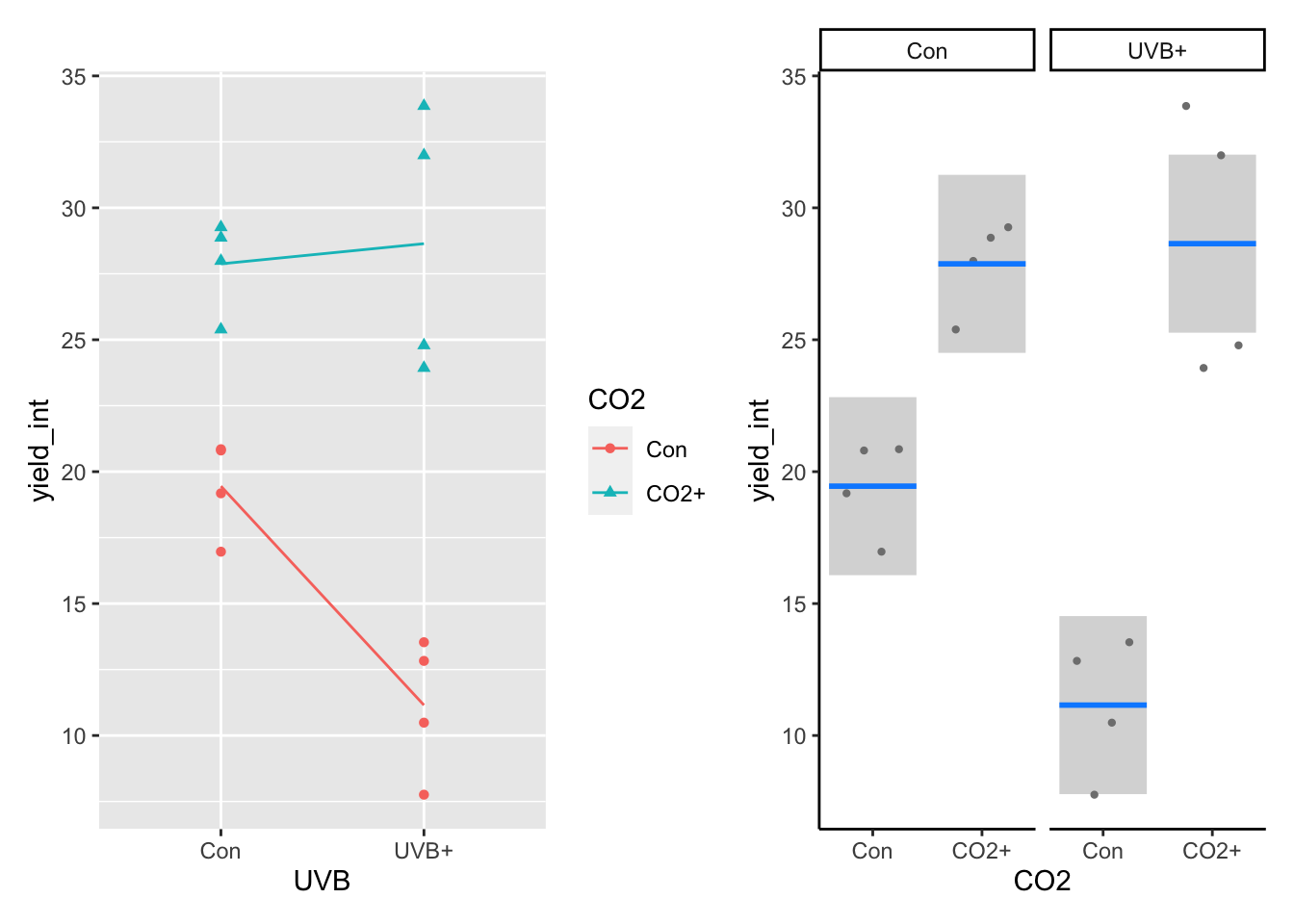
Don’t forget that the correct standard error for the ‘result’ is the residuals mean squared. You can use the dplyr + ggplot2 method, or visreg to estimate these. Here we use the visreg package and put the figure next to our original ggplot for the interaction data. Either of these would be OK for presentation, and most would opt for the left panel. Note the use of the the correct model for the design and question (model 2).
p3 <- visreg(int_mod_2,"CO2",by="UVB", gg=TRUE) +
  theme_classic()

p2+p3